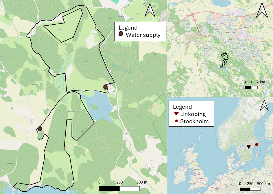
Study Area
The study was conducted in two pastures, Vattenåkarebacken (61ha) and Långbacken (46 ha), in Tinnerö, Sweden. Tinnerö is located outside of Linköping and was used for military trainings in the past. It is now a nature reserve with diverse vegetation and landscape characteristics. The open grassland areas are intersected by shrub clusters of hazel (Coryllus avelana) and hawthorn (Crategus spec.) or singular old wide crowned trees (Quercus petrea, Tilia cordata and Malus sylvestris). Besides this, both pastures have wooded areas of dense pure pine (Pinus syllvestris) mixed with spruce (Picea abies) and juniper (Juniperus communis), as well as lesser dense mixed leave broad forests of mostly oak and hazel, with singular birches (Betula pendula) mixed in.
Methods
Data collection
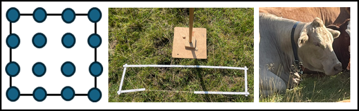
The vegetation on site was assed and mapped out using 16 plots of 0.2 x 1m per hectare, with an approximate distance of 33 m between them. In each plot all herb species were identified. Additionally, the cow dung within a radius of 5 m form each plot were counted. The vegetation height was accessed 4 times during the study period (three times during the grazing season from 17 July until 16. September) and once after season in the first two weeks of November.
17 out of 62 cows that grazed in the pastures were tracked using GPS tracking collars that transmitted the GPS position every 10-15 minutes.
Data Analysis
The collected data was processed and analysed in RStudio.
Data processing
Based on the collected point data, the cows were classified into grazing, resting and traveling, by calculating the distance in meters per minute between two consecutive time points for each cow. For each behaviour activity a threshold was set. A distance per minute less than 5m the cow was classified as resting, with a distance between 5-30 meters per minute the cow was grazing and everything above 30m per minutes was classified as traveling. For further analysis only resting and grazing were considered.
Using this classified cow data, grid-based density data were calculated by summarizing the cattle points within a grid-cell in total, per day and per hour. This data was visualised in grid-based spatial density maps and used for further spatial analysis.
A similar procedure was employed for the processing of the environmental factor data after extracting the average value of the site factors (canopy cover, soil moisture and elevation) were extracted from pre-existing raster layers. The self-collected data was assessed by calculating the average per grid cell as well.
Statistically analysis
The data were analysed in singular negative binomial regression models to test the relationships between cattle density (for both grazing and resting, respectively) and environmental factors. The environmental factors (tree and shrub cover, species richness, indicator species richness and terrain roughness index) were tested for a linear relationship, while the environmental factors (vegetation height and soil moisture) were tested with a standardised model, as a non-linear relationship was expected. Additionally, the daily grazing cattle count was tested against all environmental factors within a multi-factor negative binominal model.
To test weather specific responses the temperature and precipitation data was added separately to the regression model of tree cover, shrub cover and soil moisture, for both hourly grazing and resting cattle count. Negative binominal regression models of the proportions of the daily cow count of both behaviours against the environmental factors were used to test for behaviour specific differences.
To study the relationship between cow dung density and grazing cattle density the differences in their proportion per grid cell was calculated and visualised in a spatial grid based density map. To further investigate the relationship of nutrient transfer and species richness, the avaerge species richness and indicator species richness was tested in singular negative binomial regression models against the difference in the porportion of cow dung and grazing cattle density.
In addition, the average vegetation height of each measurement step (midseason 1, midseason 2, midseason 3 and after season) per grid cell was calculated and the differences over time were visualised in form of a boxplot-graph to highlight the variance and development during the study season.